By Trym Sorum

In this article, I will share my key insights from the StatsBomb workshop on how to use and filter their data effectively. Additionally, I will provide an example of a ‘pass map’ from the Euros Final.

1. Import Necessary Packages

First, we need to import the essential packages for downloading and working with football data.

• statsbombpy: This package enables us to download football data seamlessly.
• pandas: This package allows us to manipulate the dataset efficiently, creating rows and columns similar to Excel.
• mplsoccer: This package simplifies the process of creating football pitches with just a few lines of code.
• matplotlib: This package is used for creating visualizations and graphs in Python.

#import packages
from statsbombpy import sb
import pandas as pd
from mplsoccer import Pitch
from mplsoccer import VerticalPitch,Pitch

from highlight_text import ax_text, fig_text
from matplotlib.colors import LinearSegmentedColormap
import matplotlib.pyplot as plt
import matplotlib.patheffects as path_effects
import seaborn as sns

Lets look at how we can access StatsBombs free database of competitions and matches:

2. Call Statsbomb API

#call statsbombpy API to get all free competitions
free_comps = sb.competitions()

#print a list of free competitions
free_comps

When running the code above, you will retrieve a list of all the free competitions available through the StatsBomb open API. Each competition or season is identified by a competition_id and a season_id, which you can use to access the specific competition you're interested in. For this example, we want to select the recent EUROS 2024.

2.1 Selecting Competition

#call the statsbombpy API to get a list of matches for a given competition
#Euro 2024 competition id = 55, season id = 282
euro_2024_matches = sb.matches(competition_id=55, season_id=282)

#print the first 5 matches listed
euro_2024_matches.head(5)

Similar to how we previously called the competitions, we now call the matches from the StatsBomb API, using the competition_id and season_id for the chosen competition. We’ll save the matches as a variable named `euro_2024_matches`. Next, we need to select a specific match from the dataset. To do this, we’ll use the match_id to call the desired match.

2.2 Call specific match

#call the statsbombpy events API to bring in the event data for the match
events_df = sb.events(match_id=3943043)

#print the first 5 rows of data
events_df.head(5)

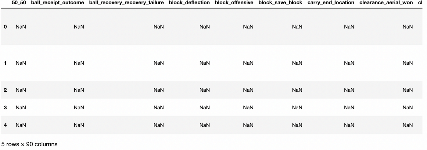
In the image above, we can see all the event data from the final between Spain and England. The dataset includes 5 rows and 90 columns, though only some of these columns are visible in the picture. There are several useful commands we can use to explore the dataset further.

3. Explore the Dataset

#print a list of columns available in the event data
events_df.columns

Index(['50_50', 'ball_receipt_outcome', 'ball_recovery_recovery_failure',
       'block_deflection', 'block_offensive', 'block_save_block',
       'carry_end_location', 'clearance_aerial_won', 'clearance_body_part',
       'clearance_head', 'clearance_left_foot', 'clearance_right_foot',
       'counterpress', 'dribble_nutmeg', 'dribble_outcome', 'dribble_overrun',
       'duel_outcome', 'duel_type', 'duration', 'foul_committed_advantage',
       'foul_committed_card', 'foul_committed_offensive', 'foul_won_advantage',
       'foul_won_defensive', 'goalkeeper_body_part', 'goalkeeper_end_location',
       'goalkeeper_outcome', 'goalkeeper_position', 'goalkeeper_technique',
       'goalkeeper_type', 'id', 'index', 'injury_stoppage_in_chain',
       'interception_outcome', 'location', 'match_id', 'minute', 'off_camera',
       'out', 'pass_aerial_won', 'pass_angle', 'pass_assisted_shot_id',
       'pass_body_part', 'pass_cross', 'pass_cut_back', 'pass_end_location',
       'pass_goal_assist', 'pass_height', 'pass_inswinging', 'pass_length',
       'pass_no_touch', 'pass_outcome', 'pass_outswinging', 'pass_recipient',
       'pass_recipient_id', 'pass_shot_assist', 'pass_switch',
       'pass_technique', 'pass_through_ball', 'pass_type', 'period',
       'play_pattern', 'player', 'player_id', 'position', 'possession',
       'possession_team', 'possession_team_id', 'related_events', 'second',
       'shot_aerial_won', 'shot_body_part', 'shot_deflected',
       'shot_end_location', 'shot_first_time', 'shot_freeze_frame',
       'shot_key_pass_id', 'shot_one_on_one', 'shot_outcome',
       'shot_statsbomb_xg', 'shot_technique', 'shot_type',
       'substitution_outcome', 'substitution_replacement', 'tactics', 'team',
       'team_id', 'timestamp', 'type', 'under_pressure'],
      dtype='object')

Using the command df.columns or, in this case, events_df.columns, we can retrieve a list of all the columns in the dataset. This helps us identify which events we are interested in examining more closely. Here are a few useful columns we can focus on:

• type: Refers to the type of action (e.g., passes, shots)
• shot_statsbomb_xg: Expected goal values
• team: Identifies the home and away teams
• player: Lists all players, both home and away
• location: Provides the x and y coordinates for events
• pass_assisted_shot_id: Represents a "key pass" (an assist leading to a shot)

To explore a specific column in more detail, we can use the unique command. Let's find all the players who played in the final by using this command:

#List of all players
events_df.player.unique()

array([nan, 'Kobbie Mainoo', 'Jordan Pickford', 'Unai Simón Mendibil',
       'Robin Aime Robert Le Normand', 'Daniel Carvajal Ramos',
       'Álvaro Borja Morata Martín', 'Daniel Olmo Carvajal',
       'Jude Bellingham', 'Rodrigo Hernández Cascante', 'Aymeric Laporte',
       'Luke Shaw', 'Declan Rice', 'Marc Guehi', 'Phil Foden',
       'Kyle Walker', 'Lamine Yamal Nasraoui Ebana',
       'Marc Cucurella Saseta', 'Nicholas Williams Arthuer', 'Harry Kane',
       'Bukayo Saka', 'Fabián Ruiz Peña', 'John Stones',
       'Martín Zubimendi Ibáñez', 'Cole Palmer', 'Mikel Oyarzabal Ugarte',
       'José Ignacio Fernández Iglesias', 'Ollie Watkins', 'Ivan Toney',
       'Mikel Merino Zazón'], dtype=object)

Notice that some players have middle names or extra last names. When referring to players in the code, it’s important to use the full names as listed in the dataset.

4. Creating a visualization: Team Pass Map

#separate start and end locations from coordinates
events_df[['x', 'y']] = events_df['location'].apply(pd.Series)
events_df[['pass_end_x', 'pass_end_y']] = events_df['pass_end_location'].apply(pd.Series)
events_df[['carry_end_x', 'carry_end_y']] = events_df['carry_end_location'].apply(pd.Series)

#create a variable for the team you want to look into
team="Spain"

#filter for only matches that the focus team played in
matches_df = euro_2024_matches[(euro_2024_matches['home_team'] == team)|(euro_2024_matches['away_team'] == team)]

#filter for events done by the focus team
#filter by event type to get only passes
#filter for passes that started outside of the final third
#filter for passes that ended in the final third
#filter for completed passes
passes_df=events_df[(events_df.team==team)&(events_df.type=="Pass")&(events_df.x<80)&(events_df.pass_end_x>80)&(events_df.pass_outcome.isna())]

#Visualize for a team
pass_colour='#e21017'

#set up the pitch
pitch = Pitch(pitch_type='statsbomb', pitch_color='white', line_zorder=2, line_color='black')
fig, ax = pitch.draw(figsize=(16, 11),constrained_layout=True, tight_layout=False)
fig.set_facecolor('white')

#plot the passes
pitch.arrows(passes_df.x, passes_df.y,
passes_df.pass_end_x, passes_df.pass_end_y, width=3,
headwidth=8, headlength=5, color=pass_colour, ax=ax, zorder=2, label = "Pass")

#plot the legend
ax.legend(facecolor='white', handlelength=5, edgecolor='None', fontsize=20, loc='best')

#set title of viz
ax_title = ax.set_title(f'{team} Progressions into Final 3rd: Euros Final', fontsize=30,color='black')

4.1 Creating Visualization: Player Pass Map

#Visualize for a given player

player_name="Fabián Ruiz Peña"

player_passes=events_df[(events_df.player==player_name)&(events_df.type=="Pass")&(events_df.x<80)&(events_df.pass_end_x>80)&(events_df.pass_outcome.isna())]

pass_colour='#e21017'

#set up the pitch
pitch = Pitch(pitch_type='statsbomb', pitch_color='white', line_zorder=2, line_color='black')
fig, ax = pitch.draw(figsize=(16, 11),constrained_layout=True, tight_layout=False)
fig.set_facecolor('white')

#plot the passes
pitch.arrows(player_passes.x, player_passes.y,
player_passes.pass_end_x, player_passes.pass_end_y, width=3,
headwidth=8, headlength=5, color=pass_colour, ax=ax, zorder=2, label = "Pass")

#plot the legend
ax.legend(facecolor='white', handlelength=5, edgecolor='None', fontsize=20, loc='best')

#set title of viz
ax_title = ax.set_title(f'{player_name} Progressions into Final 3rd', fontsize=30,color='black')

5. Summary

In relatively few lines of code, we have created a ‘passmap’ for Spain and a ‘player passmap’ for Fabián Ruiz. Analyzing these visualizations, we can see that Spain’s progressive passes were distributed across both sides of the pitch. Fabián Ruiz, in particular, operated mostly on the left side with his progressive passes, likely aiming to play in Nico Williams.

Credit goes to StatsBomb for making it so easy to work with their data, and a big thank you for hosting free webinars and workshops. These sessions provided valuable guidance on building code in a logical structure. Most of the code here is derived from their webinar, where they demonstrated various setups and visualizations. I have adapted and organized the code slightly differently to highlight some of the most valuable insights.

Source: StatsBomb Free Python Webinar (July, 2024)